Stefano J. Attardi
February 12, 2018
This is the story of how I trained a simple neural network to solve a well-defined yet novel challenge in a real iOS app. The problem is unique, but most of what I cover should apply to any task in any iOS app. That’s the beauty of neural networks.
I’ll walk you through every step, from problem all the way to App Store. On the way we’ll take a quick detour into an alternative approach using simple math (fail), through tool building, dataset generation, neural network architecting, and PyTorch training. We’ll endure the treacherous CoreML model converting to finally reach the React Native UI.
If this feels like too long a journey, not to worry. You can click the left side of this page to skip around. And if you’re just looking for a tl;dr, here are some links: code, test UI, iOS app , and my Twitter.
The Challenge
I recently built a little iOS app for mechanical watch fanciers to track the accuracy of their watches over time.
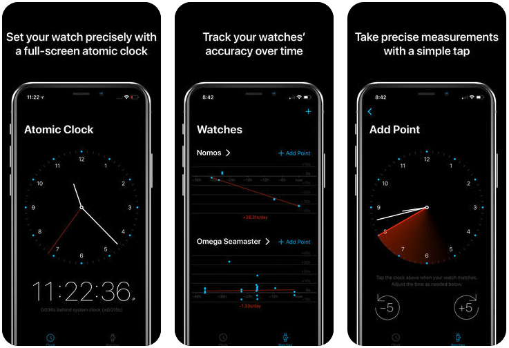
Movement - Watch Tracker introducing itself in the App Store.
In the app, watch owners add measurements by tapping the screen when their watch shows a certain time. Over time these measurements tell the story of how each watch is performing.
Mechanical Watch Rabbit Hole
If you don’t own a mechanical watch, you may be thinking: what’s the point? The point of the app? No, the point of mechanical watches! My $40 Swatch is perfectly accurate. So is my iPhone, for that matter. I see, you’re one of those. Bear with me. Just know that mechanical watches gain or lose a few seconds every day – if they’re good. Bad ones stray by a few minutes. Good or bad, they stop running if you don’t wind them. Either way you need to reset them often. And you need to service them. If they come anywhere near a magnet, they start running wild until an expert waves a special machine around them while muttering a few incantations.
True watch lovers obsess about caring for their watches, and measuring their accuracy is an importart part of the ritual. How else would you know yours is the best? Or if it needs service? It also helps in the rare case you might want to – you know – tell what time it is.
The main feature of the app is a little chart, with points plotting how your watch has deviated from current time, and trendlines estimating how your watch is doing.
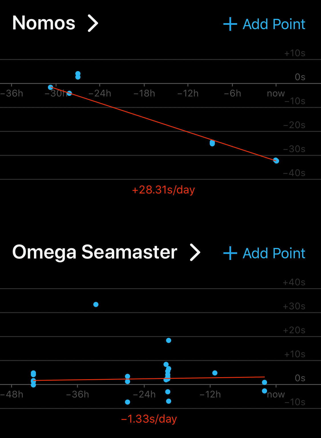
Computing a trendline given some points is easy. Use a linear regression.
However, mechanical watches need to be reset to the current time often. Maybe they drift too far from current time, or maybe you neglect a watch for a day or two, it runs out of juice, and stops. These events create a “break” in the trendline. For example:
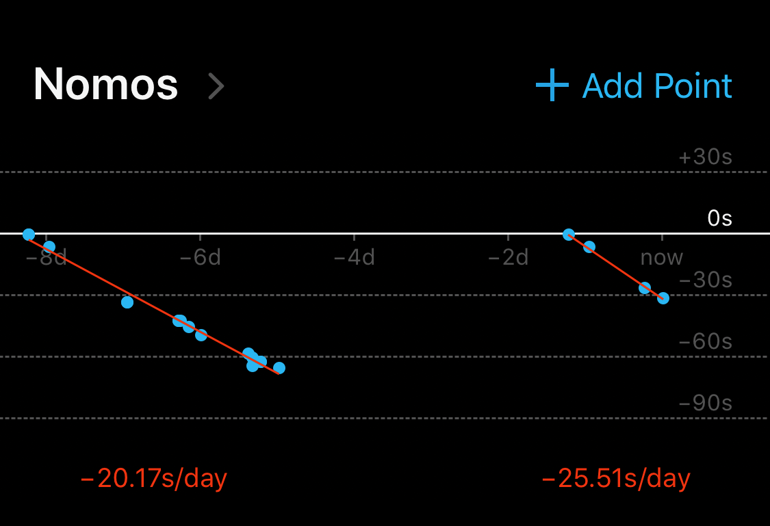
I didn’t wear that watch for a couple of days. When I picked it up again, I had to start over from zero.
I wanted the app to show separate trendlines for each of these runs, but I didn’t want my users to have to do extra work. I would automatically figure out where to split the trendlines. How hard could it be?
My plan was to Google my way out the problem, as one does. I soon found the right keywords: segmented regression, and piecewise linear regression. Then I found one person who solved this exact problem using basic math. Jackpot!
Or not. That approach tries to split the trendline at every possible point and then decides which splits to keep based on how much they improve the mean squared error. Worth a shot, I guess.
Turns out this solution is very sensitive to the parameters you pick, like how much lower the error needs to be for a split to be considered worth keeping. So I built a UI to help me tweak the parameters. You can see what it looks like here.
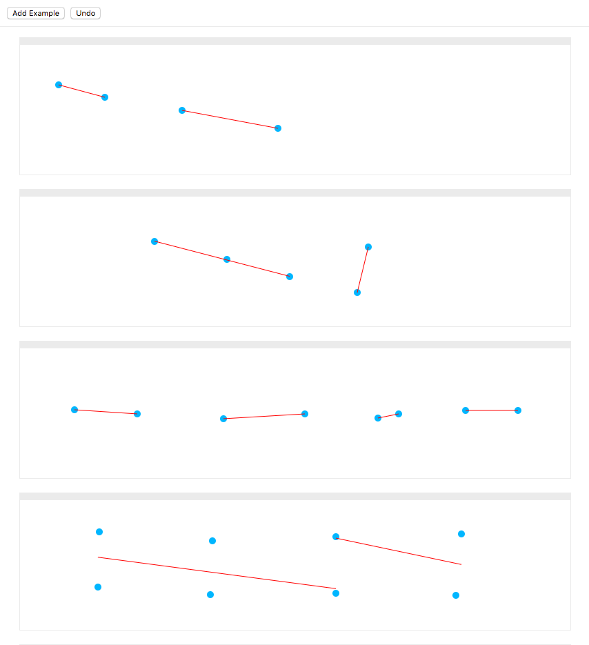
The UI I used to create and visualize examples, with hot reload for paramater tuning.
No matter how I tweaked the parameters, the algorithm was either splitting too frequently, or not frequently enough. This approach wasn’t going to cut it.
I’ve experimented for years with neural networks, but never yet had had the opportunity to use one in a shipping app. This was my chance!
The Tools
I reached for my neural networking tools. My mind was set that this would not just be another experiment, so I had one question to answer first: how would I deploy my trained model? Many tutorials sign off at the end of training and leave this part out.
This being an iOS app, the obvious answer was CoreML. It’s the only way I know of to run predictions on the GPU; last I checked CUDA was not available on iOS.
Another benefit of CoreML is that it’s built in to the OS, so I wouldn’t need to worry about compiling, linking, and shipping binaries of ML libraries with my little app.
CoreML Caveats
CoreML is quite new. It only supports a subset of all possible layers and operations. The tools that Apple ships only convert models trained with Keras. Ironically, Keras models don’t seem to perform well on CoreML. If you profile a converted Keras model you’ll notice a great deal of time spent shuffling data into Caffe operations and back. It seems likely that Apple uses Caffe internally, and Keras support was tacked on. Caffe does not strike me as a great compile target for a Keras/TensorFlow model. Especially if you’re not dealing with images.
I’d had mixed luck converting Keras models to CoreML, which is the Apple-sanctioned path (see box above), so was on the hunt for other ways to generate CoreML models. Meanwhile, I was looking for an excuse to try out PyTorch (see box below). Somewhere along the way I stumbled upon ONNX, a proposed standard exchange format for neural network models. PyTorch is supported from day one. It occurred to me to look for an ONNX to CoreML converter, and sure enough, one exists!
What about Keras and TensorFlow?
Like most people, I cut my neural teeth on TensorFlow. But my honeymoon period had ended. I was getting weary of the kitchen-sink approach to library management, the huge binaries, and the extremely slow startup times when training. TensorFlow APIs are a sprawling mess. Keras mitigates that problem somewhat, but it’s a leaky abstraction. Debugging is hard if you don’t understand how things work underneath.
PyTorch is a breath of fresh air. It’s faster to start up, which makes iterating more immediate and fun. It has a smaller API, and a simpler execution model. Unlike TensorFlow, it does not make you build a computation graph in advance, without any insight or control of how it gets executed. It feels much more like regular programming, it makes things easier to debug, and also enables more dynamic architectures – which I haven’t used yet, but a boy can dream.
I finally had all the pieces of the puzzle. I knew how I would train the network and I knew how I would deploy it on iOS. However, I knew from some of my earlier experiments that many things could still go wrong. Only one way to find out.
Gathering the Training Data
In my experience with neural networks, assembling a large-enough quality dataset to train on is the hardest part. I imagine this is why most papers and tutorials start with a well-known public dataset, like MNIST.
However, I like neural networks precisely because they can be applied to new and interesting problems. So I craft brew my own micro-datasets. Since my datasets are small, I limit myself to problems that are slightly more manageable than your run-of-the-mill Van Gogh-style portrait generation project.
Fortunately, the problem at hand is simple (or so I thought), so a small dataset should do. On top of that, it’s a visual problem, so generating data and evaluating the neural networks should be easy… given a mouse, a pair of eyes, and the right tool.
The Test UI
I had the perfect UI already. I’d built it to tweak the parameters of my simple-math algorithm and see the effects in real time. It didn’t take me long to convert it into a UI for generating training examples. I added the option to specify where I thought runs should split.
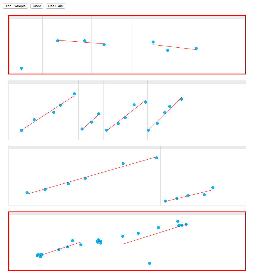
Test UI with manually-entered splits, and red boxes around incorrect predictions.
With a few clicks and a JSON.stringify call, I had enough data to jump into Python.
Parcel
As an experienced web developer, I knew building this UI as a web app with React was going to be easy. However, there was one part I was dreading, even though I’ve done it dozens of times before: configuring Webpack. So I took this as an opportunity to try Parcel. Parcel worked out-of-the-box with zero configuration. It even worked with TypeScript. And hot code reload. I was able to have a fully working web app faster than typing
create-react-app.
Preprocessing the Data
Another common hurdle when designing a neural network is finding the optimal way to encode something fuzzy, like text of varying lengths, into numbers a neural networks can understand. Thankfully, the problem at hand is numbers to begin with.
In my dataset, each example is a series of [x, y] coordinates, one for each of the points in the input. I also have a list of coordinates for each of the splits that I’ve manually entered – which is what I will be training the network to learn.
The above, as JSON, looks like this:
{ "points": [ [43, 33], [86, 69], [152, 94], [175, 118], [221, 156], [247, 38], [279, 61], [303, 89], [329, 34], [369, 56], [392, 76], [422, 119], [461, 128], [470, 34], [500, 57], [525, 93], [542, 114], [582, 138] ], "splits": [235, 320, 467]}All I had to do to feed the list of points into a neural network was to pad it to a fixed length. I picked a number that felt large enough for my app (100). So I fed the network a 100-long series of pairs of floats (a.k.a. a tensor of shape [100, 2]).
[ [43, 33], [86, 69], [152, 94], [175, 118], [221, 156], [247, 38], [279, 61], [303, 89], ...[0, 0], [0, 0], [0, 0]]The output is a series of bits, with ones marking a position where the trendline should be split. This will be in the shape [100] – i.e. array of length 100.
[0, 0, 0, 0, 1, 0, 0, 1, 0, 0, 0, 0, 1, 0, 0, 0, 0, 0, 0, ...0, 0, 0]There are only 99 possible splits, since it doesn’t make sense to split at position 100. However, keeping the length the same simplifies the neural network. I’ll ignore the final bit in the output.
As the neural network tries to approximate this series of ones and zeros, each output number will fall somewhere in-between. We can interpret those as the probability that a split should happen at a certain point, and split anywhere above a certain confidence value (typically 0.5).
[0, 0.0002, 0, 0, 1, 0, 0, 0.1057, 0, 0.002, 0, 0.3305, 0.9997, 0, 0, 0, 0, 0, ...0, 0, 0]In this example, you can see that the network is pretty confident we should split at positions 5 and 13 (correct!), but it’s not so sure about position 8 (wrong). It also thinks 12 might be a candidate, but not confident enough to call it (correct).
Encoding the Inputs
I like to factor out the data encoding logic into its own function, as I often need it in multiple places (training, evaluation, and sometimes even production).
My encode function takes a single example (a series of points of variable length), and returns a fixed-length tensor. I started with something that returned an empty tensor of the right shape:
import torch
def encode(points, padded_length=100):    input_tensor = torch.zeros([2, padded_length])    return input_tensor
Note that you can already use this to start training and running your neural network, before you put in any real data. It won’t learn anything useful, but at least you’ll know your architecture works before you invest more time into preparing your data.
Next I fill in the tensor with data:
import torch
def encode(points, padded_length=100):    input_tensor = torch.zeros([2, padded_length])    for i in range(min(padded_length, len(points))):        input_tensor[0][i] = points[i][0] * 1.0 # cast to float        input_tensor[1][i] = points[i][1] * 1.0        continue    return input_tensor
Order of Coordinates in PyTorch vs TensorFlow
If you’re paying attention, you might have noticed that the x/y coordinate comes before the position. In other words, the shape of each example is
[2, 100], not[100, 2]as you would expect – especially if you’re coming from TensorFlow. PyTorch convolutions (see later) expect coordinates in a different order: the channel (x/y in this case, r/g/b in case of an image) comes before the index of the point.
Normalization
I now have the data in a format the neural network can accept. I could stop here, but it’s good practice to normalize the inputs so that the values cluster around 0. This is where floating point numbers have the highest precision.
I find the minimum and maximum coordinates in each example and scale everything proportionally.
import torch
def encode(points, padded_length=100):    xs = [p[0] for p in points]    ys = [p[1] for p in points]
    # Find the extremes so we can scale everything    # to fit into the [-0.5, 0.5] range    min_x = min(xs)    max_x = max(xs)    min_y = min(ys)    max_y = max(ys)
    # I’m scaling y coordinates by the same ratio to keep things    # proportional (otherwise we might lose some precious information).    # This computes how much to shift scaled y values by so that    # they cluster around 0.    y_shift = ((max_y - min_y) / (max_x - min_x)) / 2.0
    # Create the tensor    input_tensor = torch.zeros([2, padded_length])
    def normalize_x(x):        return (x - min_x) / (max_x - min_x) - 0.5    def normalize_y(y):        return (y - min_y) / (max_x - min_x) - y_shift
    # Fill the tensor with normalized values    for i in range(min(padded_length, len(points))):        input_tensor[0][i] = normalize_x(points[i][0] * 1.0)        input_tensor[1][i] = normalize_y(points[i][1] * 1.0)        continue    return input_tensor
Processing Inside the Network
Many of the operations I’m writing in Python, like normalization, casting, etc., are available as operations inside most machine learning libraries. You could implement them that way, and they would be more efficient, potentially even running on the GPU. However, I found that most of these operations are not supported by CoreML.
What about Feature Engineering?
Feature engineering is the process of further massaging the input in order to give the neural network a head-start. For example, in this case I could feed it not only the
[x, y]of each point, but also the distance, horizontal and vertical gaps, and slope of the line between each pair. However, I choose to believe that my neural network can learn to compute whatever it needs out of the input. In fact, I did try feeding a bunch of derived values as input, but that did not seem to help.
The Model
Now comes the fun part, actually defining the neural network architecture. Since I’m dealing with spatial data, I reached for my favorite kind of neural network layer: the convolution.
Convolution
I think of convolution as code reuse for neural networks. A typical fully-connected layer has no concept of space and time. By using convolutions, you’re telling the neural network it can reuse what it learned across certain dimensions. In my case, it doesn’t matter where in the sequence a certain pattern occurs, the logic is the same, so I use a convolution across the time dimension.
Convolutions as Performance Optimizations
An important realization is that, though convolutions sound… convoluted, their main benefit is that they actually simplify the network. By reusing logic, networks get smaller. Smaller networks need less data and are faster to train.
What about RNNs?
Recurrent neural networks (RNNs) are popular when dealing with sequential data. Roughly speaking, instead of looking at all the input at once, they process the sequence in order, build up a “memory” of what happened before, and use that memory to decide what happens next. This makes them a great fit for any sequence. However, RNNs are more complex, and as such take more time – and more data – to train. For smaller problems like this, RNNs tend to be overkill. Plus, recent papers have shown that properly designed CNNs can achieve similar results faster than RNNs, even at tasks on which RNNs traditionally shine.
Architecture
Convolutions are very spatial, which means you need to have an excellent intuitive understanding of the shape of the data they expect as input and the shape of their output. I tend to sketch or visualize diagrams like these when I design my convolutional layers:
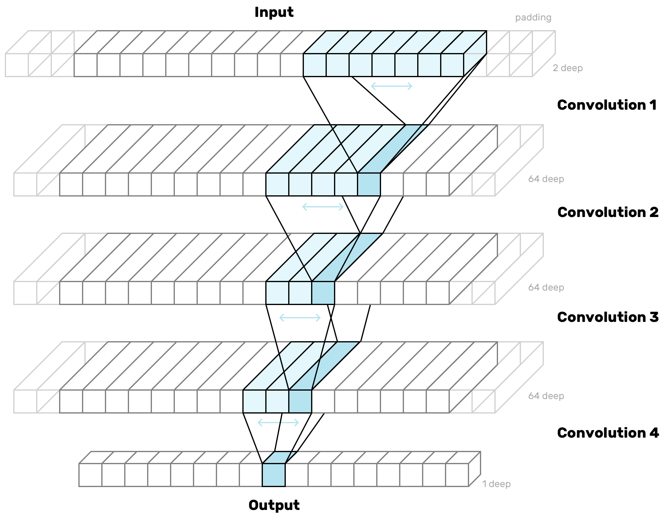
The diagram shows the shapes of the functions (a.k.a. kernels) that convert each layer into the next by sliding over the input from beginning to end, one slot at a time.
I’m stacking convolutional layers like this for two reasons. First, stacking layers in general has been shown to help networks learn progressively more abstract concepts – this is why deep learning is so popular. Second, as you can see from the diagram above, with each stack the kernels fan out, like an upside-down tree. Each bit in the output layer gets to “see” more and more of the input sequence. This is my way of giving each point in the output more information about its context.
The aim is to tweak the various parameters so the network progressively transforms the shape of the input into the shape of my output. Meanwhile I adjust the third dimension (depth) so that there’s enough “room” to carry forward just the right amount of information from the previous layers. I don’t want my layers to be too small, otherwise there might be too much information lost from the previous layers, and my network will struggle to make sense of anything. I don’t want them to be too big either, because they’ll take longer to train, and, quite likely, they’ll have enough “memory” to learn each of my examples individually, instead of being forced to create a summary that might be better at generalizing to never-before-seen examples.
No Fully-Connected Layers?
Most neural networks, even convolutional ones, use one or more “fully-connected” (a.k.a. “dense”) layers, i.e. the simplest kind of layer, where every neuron in the layer is connected to every neuron in the previous layer. The thing about dense layers is that they have no sense of space (hence the name “dense”). Any spatial information is lost. This makes them great for typical classification tasks, where your output is a series of labels for the whole input. In my case, the output is as sequential as the input. For each point in the input there’s a probability value in the output representing whether to split there. So I want to keep the spatial information all the way through. No dense layers here.
PyTorch Model
To install PyTorch, I followed the instructions on the PyTorch homepage:
pip install http://download.pytorch.org/whl/torch-0.3.0.post4-cp27-none-macosx_10_6_x86_64.whlThis is how the above structure translates to PyTorch code. I subclass nn.Module, and in the constructor I define each layer I need. I’m choosing padding values carefully to preserve the length of my input. So if I have a convolution kernel that’s 7 wide, I pad by 3 on each side so that the kernel still has room to center on the first and last positions.
import torch.nn as nn
input_channels = 2intermediate_channels = 64output_channels = 1
class Model(nn.Module):    def __init__(self):        super(Model, self).__init__()
        self.conv1 = nn.Sequential(            nn.Conv1d(in_channels=input_channels, out_channels=channels, kernel_size=7, padding=3),            nn.ReLU(),        )        self.conv2 = nn.Sequential(            nn.Conv1d(in_channels=intermediate_channels, out_channels=channels, kernel_size=5, padding=2),            nn.ReLU(),        )        self.conv3 = nn.Sequential(            nn.Conv1d(in_channels=intermediate_channels, out_channels=channels, kernel_size=3, padding=1),            nn.ReLU(),        )        self.conv4 = nn.Sequential(            nn.Conv1d(in_channels=intermediate_channels, out_channels=output_channels, kernel_size=3, padding=1),            nn.Sigmoid(),        )
All the layers use the popular ReLU activation function, except the last one which uses a sigmoid. That’s so the output values get squashed into the 0–1 range, so they fall somewhere between the ones and zeros I’m providing as target values. Conveniently, numbers in this range can be interpreted as probabilities, which is why the sigmoid activation function is popular in the final layer of neural networks designed for classification tasks.
The next step is to define a forward() method, which will actually be called on each batch of your data during training:
import torch.nn as nn
input_channels = 2intermediate_channels = 64output_channels = 1
class Model(nn.Module):    def __init__(self):        super(Model, self).__init__()
        self.conv1 = nn.Sequential(            nn.Conv1d(in_channels=input_channels, out_channels=channels, kernel_size=7, padding=3),            nn.ReLU(),        )        self.conv2 = nn.Sequential(            nn.Conv1d(in_channels=intermediate_channels, out_channels=channels, kernel_size=5, padding=2),            nn.ReLU(),        )        self.conv3 = nn.Sequential(            nn.Conv1d(in_channels=intermediate_channels, out_channels=channels, kernel_size=3, padding=1),            nn.ReLU(),        )        self.conv4 = nn.Sequential(            nn.Conv1d(in_channels=intermediate_channels, out_channels=output_channels, kernel_size=3, padding=1),            nn.Sigmoid(),        )
    def forward(self, x):        x = self.conv1(x)        x = self.conv2(x)        x = self.conv3(x)        x = self.conv4(x)        x = x.view(-1, x.size(3))        return x
The forward method feeds the data through the convolutional layers, then flattens the output and returns it.
This method is what makes PyTorch feel really different than TensorFlow. You’re writing real Python code that will actually be executed during training. If errors happen, they will happen in this function, which is code you wrote. You can even add print statements to see the data you’re getting and figure out what’s going on.
Training
To train a network in PyTorch, you create a dataset, wrap it in a data loader, then loop over it until your network has learned enough.
PyTorch Dataset
To create a dataset, I subclass Dataset and define a constructor, a __len__ method, and a __getitem__ method. The constructor is the perfect place to read in my JSON file with all the examples:
import jsonimport torchfrom torch.utils.data import Dataset
class PointsDataset(Dataset):    def __init__(self):        self.examples = json.load(open('data.json'))
I return the length in __len__:
import jsonimport torchfrom torch.utils.data import Dataset
class PointsDataset(Dataset):    def __init__(self):        self.examples = json.load(open('data.json'))
    def __len__(self):        return len(self.examples)
Finally, I return the input and output data for a single example from __getitem__. I use encode() defined earlier to encode the input. To encode the output, I create a new tensor of the right shape, fill it with zeros, and insert a 1 at every position where there should be a split.
import jsonimport torchfrom torch.utils.data import Dataset
class PointsDataset(Dataset):    def __init__(self):        self.examples = json.load(open('data.json'))
    def __len__(self):        return len(self.examples)
    def __getitem__(self, idx):        example = self.examples[idx]        input_tensor = encode(example['points'])        output_tensor = torch.zeros(100)        for split_position in example['splits']:            index = next(i for i, point in                enumerate(example['points']) if point[0] > split_position)            output_tensor[index - 1] = 1        return input_tensor, output_tensor
I then instantiate the dataset:
dataset = PointsDataset()Setting Aside a Validation Set
I need to set aside some of the data to keep track of how my learning is going. This is called a validation set. I like to automatically split out a random subset of examples for this purpose. PyTorch doesn’t provide an easy way to do that out of the box, so I used PyTorchNet. It’s not in PyPI, so I installed it straight from GitHub:
pip install git+https://github.com/pytorch/tnt.gitI shuffle the dataset right before splitting it, so that the split is random. I take out 10% of my examples for the validation dataset.
from torchnet.dataset import SplitDataset, ShuffleDataset
dataset = PointsDataset()dataset = SplitDataset(ShuffleDataset(dataset), {'train': 0.9, 'validation': 0.1})
SplitDataset will let me switch between the two datasets as I alternate between training and validation later.
Test Set
It’s customary to set aside a third set of examples, called the test set, which you never touch as you’re developing the network. The test set is used to confirm that your accuracy on the validation set was not a fluke. For now, with a dataset this small, I don’t have the luxury of keeping more data out of the training set. As for sanity checking my accuracy… running in production with real data will have to do!
PyTorch DataLoader
One more hoop to jump through. Data loaders spit out data from a dataset in batches. This is what you actually feed the neural network during training. I create a data loader for my dataset, configured to produce batches that are small and randomized.
from torchnet.dataset import SplitDataset, ShuffleDataset
dataset = PointsDataset(data_file)dataset = SplitDataset(ShuffleDataset(dataset), {'train': 0.9, 'validation': 0.1})loader = DataLoader(dataset, shuffle=True, batch_size=6)
The Training Loop
Time to start training! First I tell the model it’s time to train:
model.train()Then I start my loop. Each iteration is called an epoch. I started with a small number of epochs and then experimented to find the optimal number later.
model.train()
for epoch in range(1000):
Select our training dataset:
model.train()
for epoch in range(1000):    dataset.select('train')
Then I iterate over the whole dataset in batches. The data loader will very conveniently give me inputs and outputs for each batch. All I need to do is wrap them in a PyTorch Variable.
from torch.autograd import Variable
model.train()
for epoch in range(1000):    dataset.select('train')    for i, (inputs, target) in enumerate(loader):        inputs = Variable(inputs)        target = Variable(target)
Now I feed the model! The model spits out what it thinks the output should be.
model.train()
for epoch in range(1000):    dataset.select('train')    for i, (inputs, target) in enumerate(loader):        inputs = Variable(inputs)        target = Variable(target)
        logits = model(inputs)
After that I do some fancy math to figure out how far off the model is. Most of the complexity is so that I can ignore (“mask”) the output for points that are just padding. The interesting part is the F.mse_loss() call, which is the mean squared error between the guessed output and what the output should actually be.
model.train()
for epoch in range(1000):    dataset.select('train')    for i, (inputs, target) in enumerate(loader):        inputs = Variable(inputs)        target = Variable(target)
        logits = model(inputs)
        mask = inputs.eq(0).sum(dim=1).eq(0)        float_mask = mask.float()        masked_logits = logits.mul(float_mask)        masked_target = target.mul(float_mask)        loss = F.mse_loss(masked_logits, masked_target)
Finally, I backpropagate, i.e. take that error and use it to tweak the model to be more correct next time. I need an optimizer to do this work for me:
model.train()optimizer = torch.optim.Adam(model.parameters())
for epoch in range(1000):    dataset.select('train')    for i, (inputs, target) in enumerate(loader):        inputs = Variable(inputs)        target = Variable(target)
        logits = model(inputs)
        mask = inputs.eq(0).sum(dim=1).eq(0)        float_mask = mask.float()        masked_logits = logits.mul(float_mask)        masked_target = target.mul(float_mask)        loss = F.mse_loss(masked_logits, masked_target)
        optimizer.zero_grad()        loss.backward()        optimizer.step()
Once I’ve gone through all the batches, the epoch is over. I use the validation dataset to calculate and print out how the learning is going. Then I start over with the next epoch. The code in the evaluate() function should look familiar. It does the same work I did during training, except using the validation data and with some extra metrics.
model.train()optimizer = torch.optim.Adam(model.parameters())
for epoch in range(1000):    dataset.select('train')    for i, (inputs, target) in enumerate(loader):        inputs = Variable(inputs)        target = Variable(target)
        logits = model(inputs)
        mask = inputs.eq(0).sum(dim=1).eq(0)        float_mask = mask.float()        masked_logits = logits.mul(float_mask)        masked_target = target.mul(float_mask)        loss = F.mse_loss(logits, target)
        optimizer.zero_grad()        loss.backward()        optimizer.step()
    dataset.select('validation')    validation_loss, validation_accuracy, correct, total = evaluate(model, next(iter(loader)))
    print '\r[{:4d}] - validation loss: {:8.6f} - validation accuracy: {:6.3f}% ({}/{} correct)'.format(        epoch + 1,        validation_loss,        validation_accuracy,        correct,        total    ),    sys.stdout.flush()
def evaluate(model, data):    inputs, target = data    inputs = Variable(inputs)    target = Variable(target)    mask = inputs.eq(0).sum(dim=1).eq(0)    logits = model(inputs)    correct = int(logits.round().eq(target).mul(mask).sum().data)    total = int(mask.sum())    accuracy = 100.0 * correct / total
    float_mask = mask.float()    masked_logits = logits.mul(float_mask)    masked_target = target.mul(float_mask)    loss = F.mse_loss(logits, target)
    return float(loss), accuracy, correct, total
Time to run it. This is what the output looks like.
[ 1] validation loss: 0.084769 - validation accuracy: 86.667% (52/60 correct)[ 2] validation loss: 0.017048 - validation accuracy: 86.667% (52/60 correct)[ 3] validation loss: 0.016706 - validation accuracy: 86.667% (52/60 correct)[ 4] validation loss: 0.016682 - validation accuracy: 86.667% (52/60 correct)[ 5] validation loss: 0.016677 - validation accuracy: 86.667% (52/60 correct)[ 6] validation loss: 0.016675 - validation accuracy: 86.667% (52/60 correct)[ 7] validation loss: 0.016674 - validation accuracy: 86.667% (52/60 correct)[ 8] validation loss: 0.016674 - validation accuracy: 86.667% (52/60 correct)[ 9] validation loss: 0.016674 - validation accuracy: 86.667% (52/60 correct)[ 10] validation loss: 0.016673 - validation accuracy: 86.667% (52/60 correct)...[ 990] validation loss: 0.008275 - validation accuracy: 92.308% (48/52 correct)[ 991] validation loss: 0.008275 - validation accuracy: 92.308% (48/52 correct)[ 992] validation loss: 0.008286 - validation accuracy: 92.308% (48/52 correct)[ 993] validation loss: 0.008291 - validation accuracy: 92.308% (48/52 correct)[ 994] validation loss: 0.008282 - validation accuracy: 92.308% (48/52 correct)[ 995] validation loss: 0.008292 - validation accuracy: 92.308% (48/52 correct)[ 996] validation loss: 0.008293 - validation accuracy: 92.308% (48/52 correct)[ 997] validation loss: 0.008297 - validation accuracy: 92.308% (48/52 correct)[ 998] validation loss: 0.008345 - validation accuracy: 92.308% (48/52 correct)[ 999] validation loss: 0.008338 - validation accuracy: 92.308% (48/52 correct)[1000] validation loss: 0.008318 - validation accuracy: 92.308% (48/52 correct)As you can see the network learns pretty quickly. In this particular run, the accuracy on the validation set was already at 87% at the end of the first epoch, peaked at 94% around epoch 220, then settled at around 92%. (I probably could have stopped it sooner.)
Spot Instances
This network is small enough to train in a couple of minutes on my poor old first-generation Macbook Adorable. For training larger networks, nothing beats the price/performance ratio of an AWS GPU-optimized spot instance. If you do a lot of machine learning and can’t afford a Tesla, you owe it to yourself to write a little script to spin up an instance and run training on it. There are great AMIs available that come with everything required, including CUDA.
Evaluating
My accuracy results were pretty decent out of the gate. To truly understand how the network was performing, I fed the output of the network back into the test UI, so I could visualize how it succeeded and how it failed.
There were many difficult examples where it was spot on, and it made me a proud daddy:
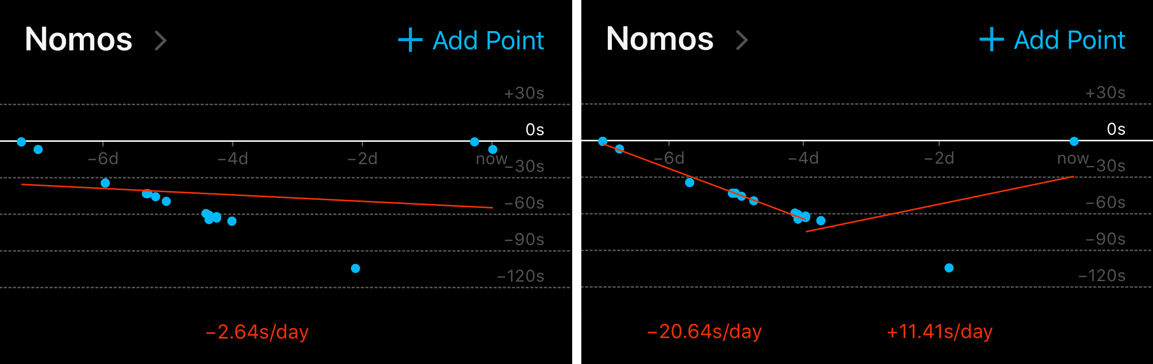
As the network got better, I started thinking up more and more evil examples. Like this pair:
I soon realized that the problem was way harder than I had imagined. Still, the network did well. It got to the point where I would cook up examples I was not be sure how to split myself. I would trust the network to figure it out. Like with this crazy one:
Even when it “fails”, according to my arbitrary inputs, it’s arguably just as correct as I am. Sometimes it even makes me question my own judgment. Like, what was I thinking here?
No, it’s not perfect. Here’s an example where it clearly fails. I forgive it though: I might have made that mistake myself.
I’m quite satisfied with these results. I’m cheating a little bit here, since most of these examples I’ve already used to train the network. Running in the app on real data will be the real test. Still, this looks much more promising than the simple approach I used earlier. Time to ship it!
Deploying
Adapting to ONNX/CoreML
I’m not gonna lie, this was the scariest part. The conversion to CoreML is a minefield covered in roadblocks and littered with pitfalls. I came close to giving up here.
My first struggle was getting all the types right. On my first few tries I fed the network integers (such is my input data), but some type cast was causing the CoreML conversion to fail. In this case I worked around it by explicitly casting my inputs to floats during preprocessing. With other networks – especially ones that use embeddings – I haven’t been so lucky.
Another issue I ran into is that ONNX-CoreML does not support 1D convolutions, the kind I use. Despite being simpler, 1D convolutions are always the underdog, because working with text and sequences is not as cool as working with images. Thankfully, it’s pretty easy to reshape my data to add an extra bogus dimension. I changed the model to use 2D convolutions, and I used the view() method on the input tensor to reshape the data to match what the 2D convolutions expect.
import torch.nn as nn
input_channels = 2intermediate_channels = 64
class Model(nn.Module):    def __init__(self):        super(Model, self).__init__()
        self.conv1 = nn.Sequential(            nn.Conv2d(in_channels=input_channels, out_channels=channels, kernel_size=(1, 7), padding=(0, 3)),            nn.ReLU(),        )        self.conv2 = nn.Sequential(            nn.Conv2d(in_channels=intermediate_channels, out_channels=channels, kernel_size=(1, 5), padding=(0, 2)),            nn.ReLU(),        )        self.conv3 = nn.Sequential(            nn.Conv2d(in_channels=intermediate_channels, out_channels=channels, kernel_size=(1, 3), padding=(0, 1)),            nn.ReLU(),        )        self.conv4 = nn.Sequential(            nn.Conv2d(in_channels=intermediate_channels, out_channels=1, kernel_size=(1, 3), padding=(0, 1)),            nn.Sigmoid(),        )
    def forward(self, x):        x = x.view(-1, x.size(1), 1, x.size(2))        x = self.conv1(x)        x = self.conv2(x)        x = self.conv3(x)        x = self.conv4(x)        x = x.view(-1, x.size(3))        return x
ONNX
Once those tweaks were done, I was finally able to export the trained model as CoreML, through ONNX. To export as ONNX, I called the export function with an example of what the input would look like.
import torchfrom torch.autograd import Variable
dummy_input = Variable(torch.FloatTensor(1, 2, 100)) # 1 will be the batch size in productiontorch.onnx.export(model, dummy_input, 'SplitModel.proto', verbose=True)
ONNX-CoreML
To convert the ONNX model to CoreML, I used ONNX-CoreML.
The version of ONNX-CoreML on PyPI is broken, so I installed the latest version straight from GitHub:
pip install git+https://github.com/onnx/onnx-coreml.gitMakefile
I love writing Makefiles. They’re like READMEs, but easier to run. I need a few dependencies for this project, many of which have unusual install procedures. I also like to use
virtualenvto install Python libraries, but I don’t want to have to remember to activate it. This Makefile does all the above for me. I just runmake train.
I load the ONNX model back in:
import torchfrom torch.autograd import Variableimport onnx
dummy_input = Variable(torch.FloatTensor(1, 2, 100))torch.onnx.export(model, dummy_input, 'SplitModel.proto', verbose=True)model = onnx.load('SplitModel.proto')
And convert it to a CoreML model:
import torchfrom torch.autograd import Variableimport onnxfrom onnx_coreml import convert
dummy_input = Variable(torch.FloatTensor(1, 2, 100))torch.onnx.export(model, dummy_input, 'SplitModel.proto', verbose=True)model = onnx.load('SplitModel.proto')coreml_model = convert(    model,    'classifier',    image_input_names=['input'],    image_output_names=['output'],    class_labels=[i for i in range(100)],)
Finally, I save the CoreML model to a file:
import torchfrom torch.autograd import Variableimport onnxfrom onnx_coreml import convert
dummy_input = Variable(torch.FloatTensor(1, 2, 100))torch.onnx.export(model, dummy_input, 'SplitModel.proto', verbose=True)model = onnx.load('SplitModel.proto')coreml_model = convert(    model,    'classifier',    image_input_names=['input'],    image_output_names=['output'],    class_labels=[i for i in range(100)],)coreml_model.save('SplitModel.mlmodel')
CoreML
Once I had a trained CoreML model, I was ready to drag the model into Xcode:
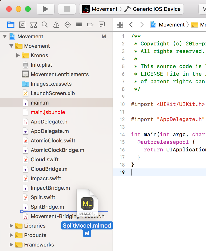
Next step was to run it, so here comes the Swift code! First, I make sure I’m running on iOS 11 or greater.
import CoreML
func split(points: [[Float32]]) -> [Int]? {  if #available(iOS 11.0, *) {
  } else {    return nil  }}
Then I create a MLMultiArray and fill it with the input data. To do so I had to port over the encode() logic from earlier. The Swift API for CoreML is obviously designed for Objective-C, hence all the awkward type conversions. Fix it, Apple, kthx.
import CoreML
func split(points: [[Float32]]) -> [Int]? {  if #available(iOS 11.0, *) {    let data = try! MLMultiArray(shape: [1, 2, 100], dataType: .float32)    let xs = points.map { $0[0] }    let ys = points.map { $0[1] }    let minX = xs.min()!    let maxX = xs.max()!    let minY = ys.min()!    let maxY = ys.max()!    let yShift = ((maxY - minY) / (maxX - minX)) / 2.0
    for (i, point) in points.enumerated() {      let doubleI = Double(i)      let x = Double((point[0] - minX) / (maxX - minX) - 0.5)      let y = Double((point[1] - minY) / (maxX - minX) - yShift)      data[[NSNumber(floatLiteral: 0), NSNumber(floatLiteral: 0), NSNumber(floatLiteral: doubleI)]] = NSNumber(floatLiteral: x)      data[[NSNumber(floatLiteral: 0), NSNumber(floatLiteral: 1), NSNumber(floatLiteral: doubleI)]] = NSNumber(floatLiteral: y)    }  } else {    return nil  }}
Finally, I instantiate and run the model. _1 and _27 are the very sad names that the input and output layers were assigned somewhere along the process. You can click on the mlmodel file in the sidebar to find out what your names are.
import CoreML
func split(points: [[Float32]]) -> [Int]? {  if #available(iOS 11.0, *) {    let data = try! MLMultiArray(shape: [1, 2, 100], dataType: .float32)    let xs = points.map { $0[0] }    let ys = points.map { $0[1] }    let minX = xs.min()!    let maxX = xs.max()!    let minY = ys.min()!    let maxY = ys.max()!    let yShift = ((maxY - minY) / (maxX - minX)) / 2.0
    for (i, point) in points.enumerated() {      let doubleI = Double(i)      let x = Double((point[0] - minX) / (maxX - minX) - 0.5)      let y = Double((point[1] - minY) / (maxX - minX) - yShift)      data[[NSNumber(floatLiteral: 0), NSNumber(floatLiteral: 0), NSNumber(floatLiteral: doubleI)]] = NSNumber(floatLiteral: x)      data[[NSNumber(floatLiteral: 0), NSNumber(floatLiteral: 1), NSNumber(floatLiteral: doubleI)]] = NSNumber(floatLiteral: y)    }
    let model = SplitModel()    let prediction = try! model.prediction(_1: data)._27  } else {    return nil  }}
I have some predictions! All I need to do is convert the probabilities into a list of indices where the probability is greater than 50%.
import CoreML
func split(points: [[Float32]]) -> [Int]? {  if #available(iOS 11.0, *) {    let data = try! MLMultiArray(shape: [1, 2, 100], dataType: .float32)    let xs = points.map { $0[0] }    let ys = points.map { $0[1] }    let minX = xs.min()!    let maxX = xs.max()!    let minY = ys.min()!    let maxY = ys.max()!    let yShift = ((maxY - minY) / (maxX - minX)) / 2.0
    for (i, point) in points.enumerated() {      let doubleI = Double(i)      let x = Double((point[0] - minX) / (maxX - minX) - 0.5)      let y = Double((point[1] - minY) / (maxX - minX) - yShift)      data[[NSNumber(floatLiteral: 0), NSNumber(floatLiteral: 0), NSNumber(floatLiteral: doubleI)]] = NSNumber(floatLiteral: x)      data[[NSNumber(floatLiteral: 0), NSNumber(floatLiteral: 1), NSNumber(floatLiteral: doubleI)]] = NSNumber(floatLiteral: y)    }
    let model = SplitModel()    let prediction = try! model.prediction(_1: data)._27
    var indices: [Int] = []    for (index, prob) in prediction {      if prob > 0.5 && index < points.count - 1 {        indices.append(Int(index))      }    }    return indices.sorted()  } else {    return nil  }}
React Native
If this were a completely native app, I would be done. But my app is written in React Native, and I wanted to be able to call this neural network from my UI code. A few more steps then.
First, I wrapped my function inside a class, and made sure it was callable from Objective-C.
import CoreML
@objc(Split)class Split: NSObject {
  @objc(split:)  func split(points: [[Float32]]) -> [Int]? {    if #available(iOS 11.0, *) {      let data = try! MLMultiArray(shape: [1, 2, 100], dataType: .float32)      let xs = points.map { $0[0] }      let ys = points.map { $0[1] }      let minX = xs.min()!      let maxX = xs.max()!      let minY = ys.min()!      let maxY = ys.max()!      let yShift = ((maxY - minY) / (maxX - minX)) / 2.0
      for (i, point) in points.enumerated() {        let doubleI = Double(i)        let x = Double((point[0] - minX) / (maxX - minX) - 0.5)        let y = Double((point[1] - minY) / (maxX - minX) - yShift)        data[[NSNumber(floatLiteral: 0), NSNumber(floatLiteral: 0), NSNumber(floatLiteral: doubleI)]] = NSNumber(floatLiteral: x)        data[[NSNumber(floatLiteral: 0), NSNumber(floatLiteral: 1), NSNumber(floatLiteral: doubleI)]] = NSNumber(floatLiteral: y)      }
      let model = SplitModel()      let prediction = try! model.prediction(_1: data)._27
      var indices: [Int] = []      for (index, prob) in prediction {        if prob > 0.5 && index < points.count - 1 {          indices.append(Int(index))        }      }      return indices.sorted()    }  } else {    return nil  }}
Then, instead of returning the output, I made it take a React Native callback.
import CoreML
@objc(Split)class Split: NSObject {
  @objc(split:callback:)  func split(points: [[Float32]], callback: RCTResponseSenderBlock) {    if #available(iOS 11.0, *) {      let data = try! MLMultiArray(shape: [1, 2, 100], dataType: .float32)      let xs = points.map { $0[0] }      let ys = points.map { $0[1] }      let minX = xs.min()!      let maxX = xs.max()!      let minY = ys.min()!      let maxY = ys.max()!      let yShift = ((maxY - minY) / (maxX - minX)) / 2.0
      for (i, point) in points.enumerated() {        let doubleI = Double(i)        let x = Double((point[0] - minX) / (maxX - minX) - 0.5)        let y = Double((point[1] - minY) / (maxX - minX) - yShift)        data[[NSNumber(floatLiteral: 0), NSNumber(floatLiteral: 0), NSNumber(floatLiteral: doubleI)]] = NSNumber(floatLiteral: x)        data[[NSNumber(floatLiteral: 0), NSNumber(floatLiteral: 1), NSNumber(floatLiteral: doubleI)]] = NSNumber(floatLiteral: y)      }
      let model = SplitModel()      let prediction = try! model.prediction(_1: data)._27
      var indices: [Int] = []      for (index, prob) in prediction {        if prob > 0.5 && index < points.count - 1 {          indices.append(Int(index))        }      }      callback([NSNull(), indices.sorted()])    } else {      callback([NSNull(), NSNull()])    }  }}
Finally, I wrote the little Objective-C wrapper required:
#import <React/RCTBridgeModule.h>
@interface RCT_EXTERN_MODULE(Split, NSObject)
RCT_EXTERN_METHOD(split:(NSArray<NSArray<NSNumber *> *> *)points callback:(RCTResponseSenderBlock *)callback)
@end
Oh, one more thing. React Native doesn’t know how to convert three-dimensional arrays, so I had to teach it:
#import <React/RCTBridgeModule.h>
@interface RCT_EXTERN_MODULE(Split, NSObject)
RCT_EXTERN_METHOD(split:(NSArray<NSArray<NSNumber *> *> *)points callback:(RCTResponseSenderBlock *)callback)
@end
#import <React/RCTConvert.h>
@interface RCTConvert (RCTConvertNSNumberArrayArray)@end
@implementation RCTConvert (RCTConvertNSNumberArrayArray)+ (NSArray<NSArray<NSNumber *> *> *)NSNumberArrayArray:(id)json{  return RCTConvertArrayValue(@selector(NSNumberArray:), json);}@end
With all this out of the way, calling into CoreML from the JavaScript UI code is easy:
import {NativeModules} from 'react-native';const {Split} = NativeModules;
Split.split(points, (err, splits) => {  if (err) return;  // Use the splits here});
And with that, the app is ready for App Store review!
Final Words
Closing the Loop
I’m quite satisfied with how the neural network is performing in production. It’s not perfect, but the cool thing is that it can keep improving without me having to write any more code. All it needs is more data. One day I hope to build a way for users to submit their own examples to the training set, and thus fully close the feedback loop of continuous improvement.
Your Turn
I hope you enjoyed this end-to-end walkthrough of how I took a neural network all the way from idea to App Store. I covered a lot, so I hope you found value in at least parts of it.
I hope this inspires you to start sprinkling neural nets into your apps as well, even if you’re working on something less ambitious than digital assistants or self-driving cars. I can’t wait to see what creative uses you will make of neural networks!
Calls to Action!
Pick one. Or two. Or all. I don’t care. You do you:
- Get the app, or tell a watch lover friend.
- Comment on Hacker News, or ask me a question on Twitter (steadicat).
- Check out the full code on GitHub.
- See the training data and try out the test UI here.
- Come up with one problem in your app that you can solve with neural networks.
- Follow me on Twitter: steadicat. I will announce future posts there.
You can also hire me as a consultant. I specialize in React, React Native, and ML work.
Thanks to Casey Muller, Ana Muller, Beau Hartshorne, Giuseppe Attardi, and Maria Simi for reading drafts of this.